How to Use VLOOKUP in Excel

If you’ve ever needed to pull a price, an email, or an order status out of one big spreadsheet and into another, you know what it takes: scrolling back and forth, copying cells one at a time, etc. VLOOKUP is the Excel function that can return the matching value for you instantly.

Learning how to do a VLOOKUP in Excel takes about five minutes, and this guide covers all of it: the exact formula and what each part means, how to look up data across two sheets, how to match on more than one condition, and how to fix the #N/A and #REF! errors that catch almost everyone at first.

If you're more of a visual learner, here's a quick video guide on how to do it: 

What’s VLOOKUP in Excel?

VLOOKUP is actually short for vertical lookup. It’s an Excel function that searches for a value in the first column of a range and returns a value from another column in the same row.

Think of it like looking someone up in a phone directory. You know the name, you scan down the name column until you find it, then read across to get the number. VLOOKUP does that scan-and-read for you. The "vertical" part matters because it searches down a column, from top to bottom, and stops at the first match.

Here is the example we will use throughout this guide. Say you have a price list with three columns, like this:

	A (Product ID)	B (Product Name)	C (Price)
Row 2	1001	Wireless mouse	$18
Row 3	1002	Keyboard	$32
Row 4	1003	Monitor stand	$45

Now, you type the keyboard’s ID (1002) into, let’s say, cell E2, because you need to know its price. You do this with the help of VLOOKUP. It takes the ID you mentioned in E2 and scans down column A until it finds a row that starts with 1002. Then, it returns the price in that same row, which is $32. In this way, you get the answer straight away, without scrolling the list and reading it off yourself.

Important: VLOOKUP never changes or moves your data. It only reads and returns. And it only looks to the right of the column it searches, which is the single most important downside to know.

VLOOKUP syntax: the four arguments explained

Every VLOOKUP formula has the same four parts, so the Excel VLOOKUP function is really just one structure you reuse. Once you know what each part does, you can write it from memory. The syntax is the following:

=VLOOKUP(lookup_value, table_array, col_index_num, [range_lookup])

Here’s what each argument means, using our example:

• lookup_value is the thing you are searching for. In our case, that is the Product ID in E2.
• table_array is the range that holds your data, starting with the column you want to search. Here, that’s A2:C100. The search column (A) has to be the first column of this range.
• col_index_num is which column of that range to return, counted from the left. Price’s in the third column of A:C, so this is 3. It’s a number, not a letter, and it counts columns inside the table array, not the worksheet.
• range_lookup is FALSE for an exact match or TRUE (or blank) for an approximate match. Use FALSE almost every time.

Put together, the finished formula is =VLOOKUP(E2, A2:C100, 3, FALSE).

A habit that saves hours: lock the table array with dollar signs, so A2:C100 becomes $A$2:$C$100. That keeps the range from shifting when you copy the formula down a column of hundreds of rows.

How to use VLOOKUP in Excel

The steps below show how to do VLOOKUP in Excel, from a blank cell to a working formula, using our price-list example again.

1. Click the cell where you want the result, for example F2.
2. Type =VLOOKUP( to start the function.
3. Click the cell holding the value you are looking up (E2), then type a comma.
4. Select the table that holds your data, from the search column across to the return column (A2:C100), press F4 to lock it to $A$2:$C$100, then type a comma.
5. Type the column number you want returned. For Unit Price, that is 3. Add a comma.
6. Type FALSE to force an exact match, then close the bracket: ).
7. Press Enter. The price appears in F2.
8. To fill the rest of the column, select F2 and double-click the small square at the bottom-right corner of the cell (see snippet below). Excel copies the formula down and matches every row.

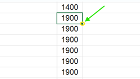
Figure 1: An illustration of where the so-called fill handle is in Excel (a small square at the bottom-right corner of a cell).

Your finished formula reads =VLOOKUP(E2, $A$2:$C$100, 3, FALSE).

Time-saving shortcut: If you don’t have time to read and apply all of what we explain here, there’s a quicker way. You can use our screen-aware assistant called Guidy. It works in the moment, pointing exactly where to click on your own screen almost like a real human. You can see more of what it does here.

How to do VLOOKUP across two sheets or workbooks

Most real-life searches require you to look into several different sheets or files. Here’s how to do a VLOOKUP between two sheets, and between two separate spreadsheets.

Two sheets in the same file

Suppose your price list lives on a sheet named Prices and you’re writing the formula on a sheet named Orders. You point the table array at the other sheet by adding its name and an exclamation mark:

=VLOOKUP(B2, Prices!$A$2:$C$100, 3, FALSE)

The easiest way to build this without typing the sheet name’s to start the formula on the Orders sheet, and when you reach the table array step, click the Prices tab and drag across the range with your mouse. Excel fills in Prices! for you.

Two separate workbooks

 Here, the reference includes the file name in square brackets:

=VLOOKUP(B2, '[PriceList.xlsx]Prices'!$A$2:$C$100, 3, FALSE)

Keep both files open while you build the formula and Excel writes that reference automatically when you click into the other workbook. If, for some reason, a sheet name contains a space, Excel wraps it in single quotes, like 'Price List'!$A$2:$C$100. That’s normal and the formula still works, so no worries.

Caution: if you close or move the source file, the link can break and show a #REF! error.

How to use VLOOKUP with multiple criteria

VLOOKUP was built to match on a single value, so having two conditions at once takes one small workaround: a helper column. Suppose you need the price for a specific product in a specific region, and the same product appears in several regions. Matching on product alone returns the wrong row. You need product plus region.

You can easily do this in three simple steps:

1. In your price list, add a new column as the leftmost column of the data (it has to be leftmost, since VLOOKUP searches the first column). Call it Key.
2. In that column, combine the two fields with a formula like =B2&"|"&C2, where B2 is the product, and C2 is the region. The "|" is just a separator so the values don’t run together.
3. Write your VLOOKUP against that combined key: =VLOOKUP(G2&"|"&H2, $A$2:$D$100, 4, FALSE); G2 and H2 are the product and region you are matching.

The helper column is a beginner-friendly way of doing this, and it works in every version of Excel. If you’d rather avoid helper columns, INDEX and MATCH or the newer XLOOKUP can handle multiple criteria with an array formula.

Exact match vs approximate match (TRUE vs FALSE)

Earlier, I mentioned that the range_lookup decides how strict the match is and getting it wrong is the most common cause of incorrect results.

FALSE (exact match) returns a result only when VLOOKUP finds the exact lookup value. If the value is not there, it returns #N/A.

TRUE or blank (approximate match) returns the closest value that’s less than or equal to your lookup value, and it assumes your first column is sorted in ascending order. If the data isn’t sorted, it can return a wrong answer with no error message at all, which makes it even worse.

When is approximate match actually useful?

Grading or banding, where you deliberately want ranges. For example, a score of 0 maps to one grade, 60 to another, 90 to another, and any score in between snaps to the band below it. That is a real use, but it’s the exception.

Safe rule for beginners: always type FALSE as the fourth argument. If you leave it out, Excel defaults to TRUE, and that’s too risky. Make FALSE a habit, and you avoid big problems in the future.

Why is my VLOOKUP not working?

I’ve answered this question many times at work. When VLOOKUP misbehaves, it’s almost always one of the following reasons.

#N/A (value not found)

The lookup value isn’t in the first column of your table, or it doesn’t match exactly. You need to look for typos and hidden trailing spaces by wrapping the lookup value in TRIM, like =VLOOKUP(TRIM(E2), ...). A very common version of this is a number stored as text and vice versa.

#REF! (invalid column)

Your col_index_num is larger than the number of columns in the table array. If your table is A:C (three columns) and you asked for column 4, Excel has nowhere to look.

Wrong value returned

You used TRUE (or left the fourth argument blank) on unsorted data. Change it to FALSE for an exact match.

Result does not fill down correctly

You didn’t lock the table array. Add dollar signs so it reads $A$2:$C$100, then copy again.

It cannot find data that is clearly there

Your lookup column isn’t the leftmost column of the range. Either move that column to the left, or switch to a function that can look left (see the next section).

One-minute solution: When Excel shows an error like #N/A or #REF! on screen, screen-aware assistant like Guidy can read what is displayed and walk you through the specific fix step by step, inside your file.

 

VLOOKUP limitations and alternatives

The errors above are mistakes you can fix. The issues below are limits built into VLOOKUP itself, where the only real fix is to switch to a different function. The key downsides of VLOOKUP are following:

• It only looks right, so the return column must be to the right of the search column, and if the value you want is to the left, VLOOKUP cannot get it.
• It breaks when columns move, because the col_index_num is a fixed number, so inserting or deleting a column inside your table quietly returns the wrong field.
• Its approximate match is the default, so forgetting FALSE may lead to wrong answers.
• It can be slow on large sheets, since each formula starts scanning from the top.

Alternatives to VLOOKUP in Excel

XLOOKUP looks in any direction, defaults to an exact match, and doesn’t break when you insert columns. If you have Excel for Microsoft 365 or Excel 2021 and later, it’s usually the better choice, and you can follow the full walkthrough on how to use XLOOKUP in Excel.

INDEX and MATCH is the classic two-function combination that works in every version of Excel, looks in any direction, and doesn’t break when columns shift.

Key takeaway

You can use VLOOKUP when your data is simple, the lookup column is on the left, and you are on an older version of Excel. And you can switch to XLOOKUP or INDEX/MATCH when you need to look left, expect your columns to change, or want to avoid the approximate-match trap.

FAQs

Why does my VLOOKUP return #N/A?

Most often the lookup value is not in the first column of your table array, or it does not match exactly. Check for typos and extra spaces (try wrapping it in TRIM), make sure numbers are not stored as text, and confirm your fourth argument is FALSE for an exact match.

What is the column index number in VLOOKUP?

It is the position of the column you want returned, counted from the left edge of your table array, where the first column is 1. It counts columns inside the range you selected, not the worksheet's column letters. If your table is A:C and you want the value in C, the index is 3.

Can VLOOKUP look to the left?

No. VLOOKUP can only return values from columns to the right of the search column. If the data you need is to the left, use INDEX and MATCH or XLOOKUP, both of which look in any direction.

Does VLOOKUP work in Google Sheets?

Yes. The syntax is the same: =VLOOKUP(lookup_value, range, index, FALSE). To pull from another Google Sheets file, combine it with IMPORTRANGE to bring in the source range first.

What is the difference between VLOOKUP and XLOOKUP?

XLOOKUP is the newer function: it looks in any direction, defaults to an exact match, and does not break when you insert columns. VLOOKUP works in every version of Excel, while XLOOKUP needs Microsoft 365, Excel 2021, or later.